Loomis-Wood windows (display functions)

The Loomis-Wood windows , which contain the so-called Loomis-Wood diagrams, are the most important part of the user interface of the LWW program in the stage of the assignment program when the predictions are not good enough to perform assignments from the Assignments window. This is because the assignment action in the LW window is not limited to the peak nearest to the prediction, but can be performed on any peak within this window.

A LW window corresponding to the active branch is most easily opened by clicking on one of the buttons numbered 1/2/3 in the lower left corner of the Branches window. Up to three LW windows can be opened simultaneously. When a LW is opened this way, the corresponding button disappears. The LW windows, which can be opened simultaneously, must have the same set of fixed upper state quantum numbers. This property is controlled internally in the program by the SeriesID, which is defined by the user in the step of Adding a new branch . It should be noted that there is no internal control of consistency of SeriesID with the fixed upper state quantum numbers and the responsibility of doing that correctly is left to the user. However, a mistake in typing the SeriesID entry can be corrected any time later by editing the particular cell in the Branches table.

There exists of course a possibility of opening a LW window by the command Draw Loomis-Wood 1/2/3 from the Loomis-Wood menu. Because the LW windows are large and it may be difficult to have them displayed without overlapping each other, a fast switching between them (bringing them on top of other windows) can be accomplished by pressing the 1/2/3 keys on the keyboard (not on the numeric pad).

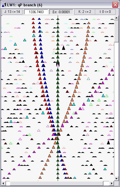
The Loomis-Wood diagram is composed of 'lines' which contain peak symbols (triangles) with positions corresponding to the wavenumbers in the neighborhood of the wavenumber predicted for a particular transition J_upper ¬ J_lower. The predicted wavenumbers for a series of J growing from top of the LW window towards the bottom are aligned along the central vertical line.

If we now assume that the vibration–rotation energies, which we use for predictions of transition wavenumbers WnCalc, are those obtained by least-squares fitting of the data corresponding to a correctly assigned vibration–rotation band, the whole series of transition wavenumbers appears along the central horizontal line. In such case, the assignment window can be easily used for making multiple assignments in one single step.

If on the other hand the prediction is not the best, the wavenumbers of the branch are displaced away from the central horizontal line, but still appear as a continuous series of symbols in the LW diagram (provided that the branch is not perturbed by a local resonance which destroys such continuous patterns).

The information about each peak appearing in the LW window is shown in the information bar (J_upper ¬ J_lower, Wavenumber, and Error = WnObs - WnCalc) as the cursor is navigated around the window. For that the user has to click somewhere in the display area of the LW window. After that he can get information on another peak by clicking on it, or navigating the cursor (a black rectangle) around the window to the nearest peak (in the direction left/right or up/down) by pressing the corresponding arrow keys on the keyboard. The position of the cursor within the LW window is sychronized with the Spectrum and Assignments windows. The peak selected in the LW window, appears in the centrum of the Spectrum window. Together with that, the corresponding line (J_upper ¬ J_lower) in the Assignments window is highlighted in yellow in the WnObs cell.